Routines

The analysis with PampelMuse is divided into several stages, each of which is performed by a different routine. The calling sequence for any of the routines is:

PampelMuse <user-configration-file> <routine>

Details about the user configuration file that has to be provided with every call can be found here. The routines that are currently available are lsted below.

PTSORT

INITFIT

Description

This first step of the analysis chain serves two main purposes. First, to determine the location of the integral field data relative to the reference catalogue. Second, to identify the subset of sources from the reference catalogue for which it is feasible to extract spectra from the IFS data. As the reference catalogue ideally was obtained from higher resolution data and typically covers a larger area on the sky, it would be impractical to try and extract a spectrum for each star in the catalogue. Instead, INITFIT uses several criteria to make a selection.

To achieve these aims, the following steps are performed:

Open the integral field data, checking their validity.

Open the reference catalogue file, checking its validity.

Create an image from the integral field data in the photometric passband in which the magnitudes in the reference catalogue are provided.

If world coordinates are available in the reference catalogue and the integral field data include sufficient information for converting world to spaxel coordinates and vice versa, compute predicted spaxel coordinates for all sources in the reference catalogue.

Create a mock image from the brightest sources in the reference catalogue, using the provided magnitudes as reference. If possible, i.e. if the previous step was carried out, the mock image is prepared using the same spatial sampling as the integral field data and the initial guess of the PSF provided in the user configuration file.

Cross-correlate the two images just created to find the most likely location of the integral field data with respect to the reference catalogue. This step is skipped if the two images have different orientation or spatial sampling.

If requested, load the PampelMuse GUI with the content following content:

The Reference view shows the mock image created from the photometric input catalogue. The sources are marked with red circles and are pickable. When selecting a source via the left mouse button, some information about it is displayed in the status bar at the bottom of the GUI. If the cross correlation carried out during the previous step was successful, then the reference view also shows the suggested position and orientation of the integral field data.

The IFS view shows a layer from datacube (initially the central one). If the cross-correlation carried out during the previous step was successful, then the GUI will show the suggested positions of the brighter sources as green circles. It is possible to grab individual spaxels from the cube using the left mouse button.

The Spectrum viewer is initially empty. If a spaxel is grabbed in the IFS view, then the spectrum of that spaxel is displayed.

From here, there are basically two options on how to proceed:

If the cross correlation was successful and you are happy with the location of the integral field data with respect to the reference catalogue, then you can just close the GUI and let INITFIT proceed with the source selection.

If the cross correlation was skipped, failed, or you are not happy with its result, then you will have to define the approximate location of the integral field data with respect to the reference catalogue manually. To do so, proceed as follows. Pick a source from the reference view with the left mouse button, then select its approximate position in the IFS view, again using the left mouse button. Once a source is successfully identified, it will be displayed by a filled red circle in the Reference view. To undo the identification for a source, pick it with the right mouse button in the Reference view. At least three sources should be identified before closing the GUI. INITFIT will then use this information to (re)determine the location of the integral field data.

Using the predicted spaxel coordinates, estimate the signal-to-noise ratio (S/N) for all sources from the reference catalogue. This also requires an estimate of the fluxes of the sources in the integral field data, i.e. the photometric zeropoint of the data must be predicted. This is done by calculating the sum of the fluxes of all sources from the reference catalogue that are inside the field of view and comparing it to the actual flux in the image created from the integral field data (cf. step 3). The photometric zeropoint is then chosen so that the two fluxes are in agreement. Depending on the size of the reference catalogue, this step may take some time, even though it is parallelized.

The next step is the actual source selection. INITFIT will loop over the sources in the reference catalogue, sorted by magnitude, i.e. brightest first, and do a number of checks to determine the status of every source in the fitting process:

Check if the local source density (given as the number of sources per resolution element, i.e per circle with radius equal to the full width at half maximum (\(\text{FWHM}\)) of the PSF) of brighter sources is below a threshold value, that is given by the configuration key initfit|confdens. As for larger fields of view, e.g. in the analysis of MUSE data, the stellar density can be very different across their extents, the confusion limit is estimated locally in an area of radius \(10\times\text{FWHM}\) around each star.

Check if S/N is above the threshold value, defined by the configuration key initfit|snrcut. In the following two cases, the S/N determined in the previous step is modified:

If a source is outside the IFS field of view, the S/N is penalized by \(\exp\{-(d/\text{FWHM})^2\}\), where \(d\) is the distance to the nearest spaxel.

If a source is nearby a brighter source (with a distance \(r<\text{FWHM}\)), the S/N is modified with the factor \(1.+0.9\log(r/\text{FWHM})\). This factor approximates the decrease in S/N found for nearby sources in [Kamann2013].

Check that there is no brighter source in the direct vicinity, defined as a circle centred of the source with a radius given by the configuration key initfit|binrad, of the source.

Sources that pass all three checks are assigned status \(2\). They are considered resolved and their spectra are set for extraction. Sources that fail the last criterion or the S/N criterion because of their vicinity to a brighter source are given status \(1\) and their contribution is accounted for in the extraction of the spectrum of the brighter neighbour. All other stars are given status \(-1\) and are ignored during the spectrum extraction.

The next step is only carried out if an unresolved stellar component should be included in the extraction process. The idea here is that the sources that are fainter than the resolution limit still create a grainy structure across the field of view (similar to surface brightness fluctuations in nearby galaxies). If the reference catalogue is of sufficient depth, this graininess can be modelled using the broadband magnitudes, positions, and the PSF. In the extraction, a combined spectrum will be extracted for the entity of these sources. If such a component is used and which sources enter it is defined by the keys in the unresolved section of the configuration. All sources included in the unresolved component are given status \(0\).

To account for the spectrum of the night sky or an unresolved stellar background, additional components may be included in the extraction. To this aim, the parameters of the sky section of the configuration can be used. The way background components are currently handled can be summarized as follows. A homogeneous grid is defined across the field of view, with a spatial sampling defined by the sky|binsize parameter. For each grid point, one additional component is included in the optimization. The weight of a spaxel in a grid point is obtained via inverse distance weighting, where distance is measured using a two-dimensional Gaussian with width \(0.5\times\texttt{binsize}\) centred on the grid point. As a rule of thumb, in crowded fields with a significant number of unresolved sources, binsize should be of the order of the spatial scale over which the stellar density changes significantly (e.g., the core radius of a star cluster).

The next step depends on the size of the IFS data, more precisely on the number of spaxels. PampelMuse was designed to handle data coming from various instruments, such as PMAS and MUSE. Now, PMAS has \(256\,\text{spaxels}\) while MUSE has more than \(90\,000\). As a consequence, the way the PSF is optimized for the two instruments is different. Within a field of view as small as the one of PMAS, you will almost never find reasonably isolated and bright stars that allow you to constrain the PSF. Instead, for PMAS-like data the idea is to optimize the PSF profile in a simultaneous fit to all resolved sources. While this approach works well for the \(\sim20\) sources which can typically be resolved in a PMAS cube, it is computationally very demanding for the \(\sim5\,000\) sources one expects to resolve in a MUSE cube. However, for MUSE data the chances of finding good PSF stars are much higher. To account for this diversity in input data, PampelMuse uses the configuration key global|smallifu. My recommendation is to set this parameter to \(\text{True}\) for cubes with less than \(\sim2\,000\,\text{spaxels}\) and to \(\text{False}\) otherwise. In the latter case, INITFIT will search for suitable sources to model the PSF during the extraction. Accepted PSF sources are those that fulfil the following criteria:

They must be brighter than the limit set by the configuration parameter initfit|psfmag.

They must have been identified as resolved (i.e. status \(2\)) in the source selection process.

They mus have a distance \(\geq \text{FWHM}\) from the edge of the observed field of view.

The relative contribution from neighbouring sources inside the region where the PSF is modelled must be smaller than a threshold value given by the configuration parameter initfit|apernois.

There are no brighter sources are allowed within a distance equal to \(1.5\times\) the PSF definition radius.

Aperture photometry is performed on each layer for each source that fulfils the above criteria. The aperture radius can be set in the configuration file. Afterwards, the centroids of the aperture photometry are used to estimate the source coordinates as a function of wavelength. In addition, the second order moments measured for the PSF sources are used to estimate the ellipticity and the position angle of the PSF (if they are free parameters in the PSF fit).

Write the results from the source selection to the dedicated multi-extension PRM-file, which is loaded by all other routines of PampelMuse.

Relevant configuration parameters

initfit|zeromagfloat: Initial guess for the photometric zeropoint of the integral field data in the provided passband, i.e. the magnitude of a source creating \(1\,\text{count}/\text{layer}\).
initfit|zerofixboolean: Flag indicating if the provided initial guess for the photometric zeropoint of the integral field data should be updated based on a comparison between the measured total flux in the data and the expected total flux given the magnitudes of the sources in the reference catalogue. Using a fixed zeropoint can be useful if the flux in the data is not dominated by the contributions of the sources listed in the reference catalogue but by the background.
initfit|confdensfloat: The confusion density, i.e. the maximum density of resolvable sources per resolution element. The local resolution limit will be the magnitude at which the density of brighter sources reaches this density. The default value of \(0.4\) was determined using simulations [Kamann2013].
initfit|snrcutfloat: The minimum estimated signal-to-noise ratio of sources that are included in the extraction.
initfit|binradfloat: The minimum spatial distance to a brighter source (in units of the PSF \(\text{FWHM}\)) of a source that is considered resolvable.
unresolved|useboolean: If True, the routine will collect all sources inside the field of view that are less than a given number of magnitudes fainter than the faintest resolved source and extract a combined spectrum for them.
unresolved|binsizefloat: The width of the magnitude interval of the unresolved component, in the sense that the faintest sources included in the unresolved component are binsize magnitudes fainter than the faintest resolved sources.
sky|useboolean: If True, one or more non-stellar components are included in the fit to account for background sources.
sky|binsizefloat: The distance between two background patches. If set to \(-1\), only a constant background is used.
initfit|psfmagfloat: The maximum magnitude of sources considered as suitable for modelling the PSF. If not given (default), the limit is \(3\) magnitudes brighter than the faintest resolved source.
initfit|apernoisfloat: The maximum allowed contamination around a PSF source from a neighbouring source. It is measured as the flux ratio of the brightest source within the PSF definition radius and the flux of the considered source itself.}
initfit|aperradfloat: The radius in spaxels of the circle around each PSF source in which the aperture photometry is performed.

SINGLESRC

CUBEFIT

Description

This routine performs the extraction of the spectra by simultaneously fitting a PSF to all sources that have been identified as resolvable by the INITFIT routine. CUBEFIT analyses the integral field data layer by layer, starting from the central layer and alternatingly proceeding into the red and the blue parts of the cube. On each layer, the code performs an iterative analysis in order to extract the optimal flux for each source. This iterative scheme, also depicted in the figure below, can be summarized as follows.

Using the initial guesses for the PSF and the coordinate transformation, a first fit of the fluxes is performed. The flux fit is a linear least-squares fit that can be solved by direct matrix inversion and does not require initial guesses. The matrix contains the PSF profiles of the individual components, one per column. As each PSF profile is significantly different from zero only in the vicinity of the represented star, the majority of the matrix entries are zero. For such sparse matrices very efficient inversion algorithms are available. CUBEFIT uses the method lsmr developed by [Fong2010], which is available in the scipy.sparse.linalg package. The performance was tested for up to \(10\,000\) sources, yielding reliable solutions in reasonable computation times.

With an initial value for all fluxes available, the spaxel coordinates and/or the PSF are optimized (if requested). The way in which this is done depends on the analysis setup, in particular on the value of the global|smallifu parameter and whether INITFIT or SINGLESRC has been used to initialize the analysis.

If INITFIT has been used and the global|smallifu parameter is enabled, the optimization is carried out using the whole layer, i.e. a model is created containing all resolvable sources and the \(\chi^2\) between this model and the layer is minimized. The optimization is performed for the parameters of the coordinate transformation first, and afterwards for the PSF parameters.

If INITFIT has been used and the global|smallifu parameter is disabled, CUBEFIT will perform a series of single-PSF fits. For each source deemed suitable, the relevant part of the layer is selected and adjacent sources are subtracted based on the current best-fit model. Afterwards, a single PSF model is fitted to the data and optimized for the flux, the centroid positions, and all free PSF parameters. Once all sources have been processed in this way, the new coordinate transformation is obtained by comparing the reference coordinates to the fitted centroids. In addition, the new PSF model is obtained by averaging the parameters obtained in the successful fits.

If SINGLESRC has been used, the process is very similar to option b., only that the centroids are used directly, given that no coordinate transformation is available.

The non-linear optimizations required to perform the steps just described are performed via the Levenberg-Marquardt algorithm scipy.optimize.least. To speed up the computation, CUBEFIT internally calculates the Jacobi matrix, i.e. the matrix containing the partial derivatives of the PSF profile(s) with respect to the fitted parameters.

The updated PSF and coordinate transformation are used to refit the fluxes of the sources. Afterwards, it is checked whether the fluxes converged. The convergence criterion that is used by PampelMuse is that the median change in flux compared to the last iteration is \(<0.005\). If the convergence criterion is fulfilled or the maximum number of iterations has been reached, the analysis is continued with the next layer. Otherwise, the iteration continues with fitting the coordinate transformation and/or PSF parameters (step 2). The maximum number of iterations can be set using the configuration key cubefit|iterations.

After all the requested layers have been analysed in this way, the results are written to the PRM-file.

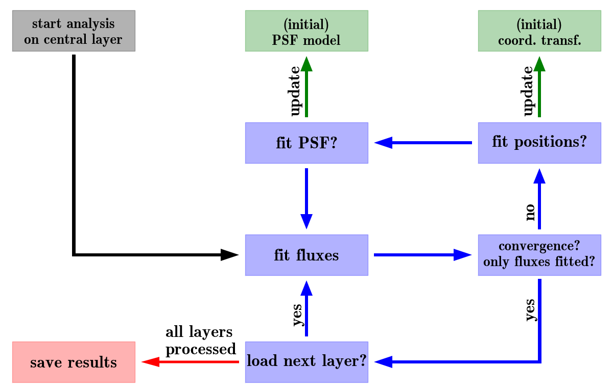
_images/cubefit_scheme.png — The iterative fitting approach of the CUBEFIT routine.

After the first two layers have been processed, the code will use the fit results for the PSF and the coordinate transformation as initial guesses for the analysis of the next layer. To avoid that a failed fit in one layer (e.g. because of a strong cosmic-ray) influences the analysis of the following ones, the initial guesses are obtained by averaging over the results from the \(10\) adjacent layers.

Note

This routine is computationally the most demanding part of PampelMuse. The executions times can vary from a few minutes if only some sources are present to tens of hours for really crowded fields and huge datasets. My recommendation is to start CUBEFIT in a screen session, detach from it and have a good glass of wine. (Note however that for budget reasons, the wine is not shipped with PampelMuse)

New in version 1.0: In cases where the astrometric accuracy of the reference catalogue is limited (e.g., because proper motions have offset the sources with respect to their reference coordinates), CUBEFIT offers the possibility to determine the shifts between the predicted and the actual coordinates of the sources. To this aim, the configuration parameter cubefit|offsets must be enabled. In this case, CUBEFIT will perform individual PSF fits for all resolved sources (in a very similar manner to the one described above in step 2b for the PSF sources, only that no PSF parameters are fitted) in order to determine their true centroid positions. The offsets with respect to their predicted centroid positions are applied in subsequent fits to the source fluxes. Averaged offsets across the wavelength range are also written to the PRM-file and used in all subsequent analysis steps.

Relevant configuration parameters

cubefit|iterationsinteger: The maximum number of iterations that is performed by CUBEFIT on an individual layer of the IFS data.
cubefit|offsetsboolean: In order to determine and correct for offsets between the source coordinates provided in the reference catalogue and the actual coordinates, this parameter must be enabled.

POLYFIT

Description

The POLYFIT routine serves two purposes. First, it allows the user to visually check the results of the analysis, by displaying the spectra extracted for individual sources or inspecting the wavelength dependencies of the spaxel coordinates or PSF parameters. Second, it provides the functionality to fit polynomial functions to the aforementioned coordinates and parameters. The idea behind the latter is that, from a theoretical point of view, you expect those properties to vary smoothly with wavelength, e.g. because of differential atmospheric refraction (DAR). However, because of the limited S/N in each layer, the values determined by CUBEFIT as a function of wavelength will show scatter, especially in spectral regions were the signal is low, such as in telluric absorption bands. Fitting those variations with polynomials averages out the scatter and should therefore lead to a higher S/N in the extracted spectra. When starting CUBEFIT again after performing the polynomial fits, it will only refit the fluxes in each layer while keeping the other parameters fixed at their polynomial values.

When running PampelMuse in interactive mode, the routine will load the PampelMuse GUI, which gives the user a number of options to work with the data:

The purpose of the Spectrum Viewer is to display extracted spectra or the wavelength dependencies of the fitted spaxel coordinates or PSF parameters. The data to be shown can be selected using the two drop-down menus labelled Data: to the bottom left of the panel. Via HDU, one can select the parameter class (spectrum, coordinate, PSF parameter) to be displayed, while Identifier lets one select a specific source ID in case a spectrum or spaxel coordinates should be displayed, or the specific parameter in case a PSF or coordinate transformation parameters should be displayed. The requested data is displayed upon clicking the green button.

Further, one can use the Spectrum Viewer to exclude wavelength ranges from the polynomial fits. To this aim, keep the left mouse button pressed while scanning over the desired range. Doing the same with the right mouse button lets you unmask regions again. If any wavelength ranges should be excluded from the fits by default (e.g. because of strong telluric absorption bands), you may specify these ranges using the configuration key polynom|mask. This key is also very helpful if POLYFIT is run in non-interactive mode (see below).

The two drop-down menus labelled Fit: to the bottom right of the Spectrum Viewer allow one to specify the type and degree of the polynomial that is used to fit the data. The default values can be set using the configuration keys polynom|type and polynom|degree. The fit is carried out via a click on the green button to the right of the drop-down menus. Note that currently only fits to the PSF parameters and the spaxel coordinates are supported. Fitting the individual spaxel coordinates instead of the coordinate transformation parameters (which were used to calculate them) is preferred because the parameters of the coordinate transformation can sometimes show correlated variations (in particular if the field of view contains only a few spaxels) that are difficult to correctly describe with polynomials.

The IFS View displays again the cube, with the positions of the extracted sources overplotted. The size of the circles used to indicate the locations of the sources scale with their brightnesses. Sources marked by green circles are used to fit the PSF. The source that is currently displayed in the Spectrum View is highlighted via a filled circle. When picking a source while the Spectrum View shows a spectrum or a spaxel coordinate, the spectrum/coordinate of the picked source will be shown. Depending on the number of sources included in the analysis, the plot can look very messy. However, you can use the standard matplotlib navigation bar located to the top right to zoom into the data or pan across it. Furthermore, you can restrict the magnitude range or the status of the sources that are displayed using the functionalities to the left of the IFS View.

The Reference View is currently not used.

After one has fitted all the desired parameters and is happy with the results, one can use the buttons to the top left of the GUI to save the results to the PRM-file.

Note

When PampelMuse is not run in interactive mode (controlled by the configuration key global|interact), POLYFIT will not show the GUI but use polynomials of the requested order to fit the source coordinates and the free PSF parameters automatically. The type and order of the polynomials being used as well as the wavelength ranges that should be masked can still be controlled via the respective configuration keys (see below).

Relevant configuration parameters

polynom|masktuple: In case any wavelength range(s) should be excluded from the polynomial fits by default, provide their start and end values. The values must be provided as a single tuple of even length, so that even indices contain the start values and odd indices the end values of the ranges to be masked.
polynom|typestring: The type of polynomial used to fit the wavelength dependencies. Can be one of plain (normal polynomial), chebyshev, legendre, and hermite.
polynom|degreeinteger: The degree of the polynomials used to fit the wavelength dependencies.

SUBTRES

Description

PampelMuse also offers the possibility to create a residuals cube once the analysis is complete. To this aim, the routine SUBTRES can be used. By default, it will subtract the contribution of all resolved stellar sources from the data cube. However, it is also possible to subtract a subset of the resolved sources, using either of the subtres|include or the subtres|exclude configuration keys. Only one of the keys should be set at a time.

In addition, SUBTRES allows the user to subtract the sky background and/or the background created by an unresolved stellar component (if either of the components has been used in the analysis). To this aim, a key subtract exists in both the sky and unresolved sections of the configuration.

Relevant configuration parameters

subtres|includetuple: The list of IDs of resolved sources that should be subtracted from the IFS data using SUBTRES. The default is to subtract all resolved sources unless the option subtres|exclude is used instead.
subtres|excludetuple: The list of IDs of resolved sources that should NOT be subtracted from the IFS data using SUBTRES. By default, all sources are subtracted unless the sources to subtract are specified using the subtres|include option instead.
sky|subtractboolean: Flag indicating if the sky background should be removed when running the SUBTRES routine.
unresolved|subtractboolean: Flag indicating if the unresolved stellar background should be removed when running the SUBTRES routine.

GETSPECTRA

Description

Once the analysis is complete, one probably wants to obtain the spectra in some other format than the PRM-file. To facilitate this, PampelMuse includes the routine GETSPECTRA It will store all the extracted spectra as individual FITS files that contain the spectrum in the primary extension and an estimate of the uncertainties in an image HDU named SIGMA. The header of each file will contain the correct dispersion information, general information about the star and the spectrum as well as a number of HIERARCH keywords copied from the PRM-file. Further details about the content of the output spectra can be found here.

This routine requires the configuration key getspectra|prefix to be set in the user configuration file. This is a string (typically the name of the observed cluster, galaxy, …) that is used as a common prefix to all FITS files that are written. Additionally, the key getspectra|folder in the same section can be used to provide a folder in which all spectra should be stored.

Relevant configuration parameters

getspectra|prefixstring: The common prefix given to all FITS files that are written.
getspectra|folderstring: The name of the folder in which the FITS files should be stored.